Estimated Reading Time: 15 minutes

In regression problems, we often model the conditional mean of a conditional probability distribution $p(\textbf{t}|\textbf{x})$ by minimizing the least squares ($L^2$-loss) between the input and target variables (this can be shown through a brief derivation using the calculus of variations). For more complicated multimodal distributions, however, using merely the conditional mean of a univariate Gaussian can prove to be problematic.

In this blog post, we show how a neural network can represent more general distributions (in our case, we fit a Gaussian mixture model) and then show how one might implement such a network in code. Such models are known as mixture density networks, and we will see how to model the errors and corresponding outputs.

Motivation

For simple regression problems, we can model the conditional distribution $p(\textbf{t}|\textbf{x})$ using a Gaussian. This can lead to disastrous results however, for outputs with non-Gaussian distributions. This can be seen, for example, in inverse problems. For a simple example, consider the example of the inverse problem in robot kinematics shown below:

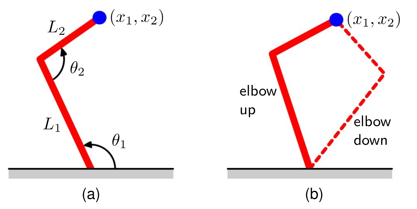
The forward problem involves finding the end-effector position of a two-link robot arm that has arm lengths $L_1$ and $L_2$, is tilted at an angle $\theta_1$ from the ground, and has an inter-arm angle of $\theta_2$. The forward problem, given the set of parameters, has a unique solution. However, the inverse problem of finding the corresponding angles $\theta_j$ and lengths $L_j$ has multiple solutions (and thus multiple modes) as shown in the second image. Similarly, other inverse problems are readily seen to be multimodal.

For example, consider a data set $\mathcal{D}$ of elements in $\mathbb{R}^2$ generated as follows: sample a set of values $\{x_n\}$ uniformly from the interval $(0,1)$ and define the corresponding target values $t_n := x_n+0.3\sin(2\pi{x}) + r(-0.1,0.1)$ where $r(-0.1,0.1)$ is some uniform noise in the range $-0.1$ to $0.1$.

import numpy as np
import matplotlib.pyplot as plt
import torch
import torch.nn as nn
from torch.utils.data import Dataset, DataLoader
from tqdm import tqdm
import torch.nn.functional as F

N = 300
rng = np.random.default_rng(19)
x = rng.random(N)
y = x + 0.3*np.sin(2*np.pi*x) + (0.2*rng.random(x.size) - 0.1)

plt.scatter(x, y, edgecolors = 'g', facecolors='none')

class train_dataset(Dataset):
    def __init__(self, x , y):
        self.x = torch.from_numpy(x).type(torch.FloatTensor)
        self.y = torch.from_numpy(y).type(torch.FloatTensor)

    def __len__(self):
        return len(self.x)

    def __getitem__(self, idx):
        return self.x[idx].unsqueeze(0), self.y[idx].unsqueeze(0)           

The forward regression problem of mapping a function $x \to t$ can readily be solved by doing maximum-likelihood under a Gaussian distribution using the standard L2-loss (say, by fitting a neural network or defining suitable basis functions and then doing linear regression). The inverse problem, however, of finding a mapping $t \to x$ leads to very poor results. We show this by fitting a neural network with two hidden layers (with 6 hidden units per hidden layer) to both problems and minimizing the L2-loss. Note we use the softplus activation $f(x)=\log(1+\exp(x))$ due to the limited number of units and layers (we wish to fit a "smooth" function like a polynomial. Using ReLUs can work too but they tend to give "harder" functions due to the limited number of connections in our chosen model).

device = 'cuda' if torch.cuda.is_available() else 'cpu'

class NeuralNet(nn.Module):
    '''
    Simple Two Layer Network with 6 hidden units.
    '''
    def __init__(self):
        super().__init__()
        self.stack = nn.Sequential(
            nn.Linear(1, 6),
            nn.Sigmoid(),
            nn.Linear(6,6),
            nn.Softplus(),
            nn.Linear(6, 1)
        )

    def forward(self, x):
        out = self.stack(x)
        return out 

forward_model = NeuralNet().to(device)
inverse_model = NeuralNet().to(device)

#hyperparameters
learning_rate_forward = 0.1
learning_rate_inverse = 0.05
batch_size = N
epochs = 2000

loss_fn = nn.MSELoss()
forward_optimizer = torch.optim.Adam(forward_model.parameters(), lr = learning_rate_forward)
inverse_optimizer = torch.optim.Adam(inverse_model.parameters(), lr = learning_rate_inverse)
train_dataloader = DataLoader(train_dataset(x, t), batch_size = batch_size, shuffle = True)

The training loop for the model can be shown as follows:

def train():
    forward_model.train()
    inverse_model.train()

    for epoch in tqdm(range(epochs)):
        forward_losstot, inverse_losstot = 0,0
        for batch, (x, t) in enumerate(train_dataloader):
            x, t = x.to(device), t.to(device)
            forward_pred = forward_model(x)
            inverse_pred = inverse_model(t)
            forward_loss = loss_fn(forward_pred, t)
            inverse_loss = loss_fn(inverse_pred, x)

            with torch.no_grad():
                forward_losstot += forward_loss.item()
                inverse_losstot += inverse_loss.item()

            forward_loss.backward()
            inverse_loss.backward()
            forward_optimizer.step()
            inverse_optimizer.step()
            forward_optimizer.zero_grad()
            inverse_optimizer.zero_grad()

        tqdm.write(f'epoch: {epoch}, forward loss: {forward_losstot}, inverse loss: {inverse_losstot}')

train()

which gives the following fits: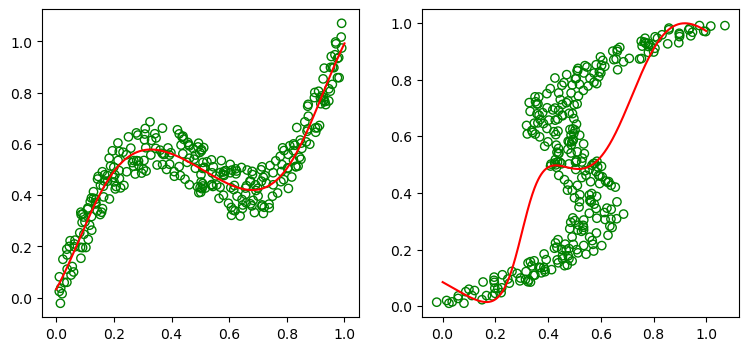

We thus see that using least squares (which corresponds to a maximum likelihood model under a Gaussian distribution using a least squares fit) gives a very poor fit for the non-Gaussian inverse problem. We thus seek a general framework for modeling conditional distributions. This can be achieved by using mixture models for the conditional distributions $p(\textbf{t}|\textbf{x})$, which can approximate probability distributions to arbitrary accuracy with enough mixtures (see [3]). These class of models are known as mixture density networks. For this blog post, we focus mainly on Gaussian Mixture Density Networks for which the subpopulations are Gaussian.

Gaussian Mixture Density Networks

Gaussian mixture density networks use neural networks to model the parameters of a conditional probability that uses a Gaussian mixture model (the components are Gaussian). Here, we assume that the Gaussians are isotropic, ie. the covariance matrices of the Gaussians are a diagonal matrix of the form $\sigma^2\textbf{I}$. That is, $$p(\textbf{t}|\textbf{x}) = \sum_{k=1}^{K} \pi_k(\textbf{x})\mathcal{N}(\textbf{t}|\mu_k(\textbf{x}), \sigma^2_k(\textbf{x}))$$ where we assume there are $K$ classes (this $K$ is a hyperparameter). Here, $\pi_k$ can be interpreted as the class-priors for class $k$, $\mu_k$ is the mean of the for class $k$ and $\sigma$ is the standard deviation of the class. Note the dependence on $\textbf{x}$ for each of the given parameters, which shows that the density parameters are dependent on the choice of input $\textbf{x}$. Such models are called heteroscedastic because of the multiple variances we model for each subpopulation.

To model the density function using a neural network, we take the outputs of the neural networks to be the various parameters of the density function, namely $\pi_k$, $\mu_k$ and $\sigma_k^2$ as illustrated below:

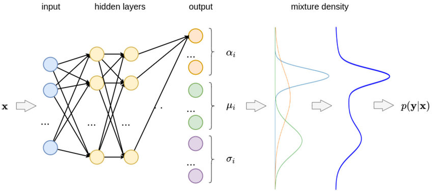
If, for example, we assume the density function has $K$ components, and the output $\textbf{t}$ has $L$ components, then the network will have as outputs:

1. Pre-activation for class priors $\pi_k$: The network has $K$ output-unit pre-activations $a_k^{\pi}$ that determine the mixing coefficients $\pi_k$. Since the mixing coefficients must satisfy $$\sum_{k=1}^{K} \pi_k(\textbf{x}) = 1, \quad 0 \le \pi_k(\textbf{x}) \le 1$$ we take the class priors $\pi_k$ to be given by using the softmax of the pre-unit activations: $$\pi_k(\textbf{x}) = \frac{\exp(a_k^{\pi})}{\sum_{l=1}^{K}\exp(a_l^{\pi})}$$
2. Pre-activation for the variances: The network has $K$ output-unit pre-activations $a_k^{\sigma}$. We must have the variances $\sigma^2_k(\textbf{x}) \ge 0$ so we take the exponentials of the pre-activations using $$\sigma_k(\textbf{x}) = \exp(a_k^{\sigma})$$
3. Pre-activation for the means: The networks has $LK$ pre-activations for the mean $a^{\mu}_{kj}$ where the mean for the $k$th Gaussian can be represented by using the pre-activations directly (so the output activations are the identity): $$\mu_k(\textbf{x}) = \begin{bmatrix} a^{\mu}_{k1}, \dots , a^{\mu}_{kL}\end{bmatrix}^{T}$$
   This gives a total of $(L+2)K$ parameters.

The learnable parameters $\textbf{w}$ of the model can be using the maximum likelihood estimate(MLE) or equivalently minimizing the negative log likelihood: $$E(\textbf{w}) = -\sum_{n=1}^{N}\ln \left\{\sum_{k=1}^{K}\pi_k(\textbf{x}_n,\textbf{w})\mathcal{N}(\textbf{t}_n|\mu_{k}(\textbf{x}_n,\textbf{w}), \sigma_k^2 (\textbf{x}_n,\textbf{w})) \right\}$$ This error function can then be optimized using standard optimizers (SGD, ADAM, etc.).

Predictive Distribution

Once a mixture density function has been trained, we have a model for the conditional density function which can be used to predict the value of the output vector for new inputs. Assuming a squared loss, one can use the calculus of variations to show the conditional mean $\mathbb{E}_t[t|x] = \int \textbf{t} p(\textbf{t}|\textbf{x})d\textbf{t}$ minimizes the loss for the regression problem. For the mixture model, we have the conditional mean is given by $$\mathbb{E}[\textbf{t}|\textbf{x}] = \sum_{k=1}^{K}\pi_k(\textbf{x})\mu_k(\textbf{x}))$$ which can be interpreted as a weighted average of the means of the component Gaussians using the class priors. Note that a mixture density network can reproduce the least squares result as a special case by approximating the conditional mean by assuming the distribution is unimodal and there is only one class (ie. $K=1$). Similarly, we can calculate $$\sigma^2(\textbf{x}) = \mathbb{E}\left[ \|\textbf{t}-\mathbb{E}[\textbf{t}|\textbf{x}]\|^2|\textbf{x}\right]=\sum_{k=1}^{K}\pi_k(\textbf{x})\left\{\sigma_k^2(\textbf{x})+\left\|\mu_k(\textbf{x})- \sum_{l=1}^{K}\pi_l(\textbf{x})\mu_l(\textbf{x})\right\|^2\right\}$$ Note, however, that for multimodal distributions the conditional mean can often give a poor representation of the data. Going back to the robot kinematics example, note that the average of the two modes (the "elbow up" and "elbow down" solutions) to the inverse problem have an average which is itself not a solution to the problem. The conditional mode, on the other hand, often gives a much better representation of the data and can be approximated by taking the mean of the component $k$ with largest prior $\pi_k$.

Let's see how this is applied in practice. We return to our toy example of data $\mathcal{D}$ defined above. Here, we assume there to be $3$ component Gaussians which corresponds to $3*3=9$ output units corresponding to the $3$ mean, variance, and prior parameters respectively. The code for the model is shown below:

class MixtureDensityNet(nn.Module):
    '''
    Two Layer mixture density network with 3 classes.
    '''

    def __init__(self, n_components):
        super().__init__()
        self.components = n_components
        self.network = nn.Sequential(
            nn.Linear(1, 5),
            nn.ReLU(),
            nn.Linear(5,5),
            nn.ReLU(),
            nn.Linear(5, self.components*3),
        )

    def forward(self, x, epsilon=1e-6):
        preact = self.network(x)
        pi = F.softmax(preact[...,:self.components], -1)
        mu = preact[...,self.components:self.components*2]
        sigma = torch.exp(preact[...,self.components*2:self.components*3] + epsilon)
        return pi, mu, sigma

    def mode(self, x):
        pi, mu, _ = self.forward(x)
        argpi = torch.argmax(pi)
        mu = torch.flatten(mu)
        return mu[argpi.item()]

We set the hyperparameters as follows:

device = 'cuda' if torch.cuda.is_available() else 'cpu'
mixture_model = MixtureDensityNet(3).to(device)

#hyperparameters
learning_rate = 0.001
batch_size = 300
epochs = 5000

optimizer = torch.optim.Adam(mixture_model.parameters(), lr=learning_rate)
dataloader = DataLoader(train_dataset(x, t), batch_size = batch_size, shuffle = False)

and define a custom loss function for the density network given by $E$ above:

class MixtureLoss(nn.Module):
    def __init__(self):
        super().__init__()

    @classmethod
    def gaussian(cls, t, mu, sigma):
        res = (t.expand_as(mu) - mu) * torch.reciprocal(sigma)
        res = -0.5 * (res * res)
        return torch.exp(res)*torch.reciprocal(sigma) * (1.0/ np.sqrt(2.0* np.pi))

    def forward(self, pred, target):
        pi, mu, sigma = pred
        result = MixtureLoss.gaussian(target, mu, sigma) * pi 
        result = torch.sum(result, dim = 1)
        result = -torch.log(result)
        return torch.mean(result)

loss_fn = MixtureLoss()

The training code is then given as follows:

def train():
    mixture_model.train()

    for epoch in tqdm(range(epochs)):
        losstot = 0
        for batch, (x, t) in enumerate(dataloader):
            x, t = x.to(device), t.to(device)
            pred = mixture_model(t)
            loss = loss_fn(pred, x)

            with torch.no_grad():
                losstot += loss.item()

            loss.backward()
            optimizer.step()
            optimizer.zero_grad()

        tqdm.write(f'epoch: {epoch}, loss: {losstot}')

train()

We then plot the mixing coefficients $\pi_k$ and means $\mu_k$ as a function of $\textbf{x}$.

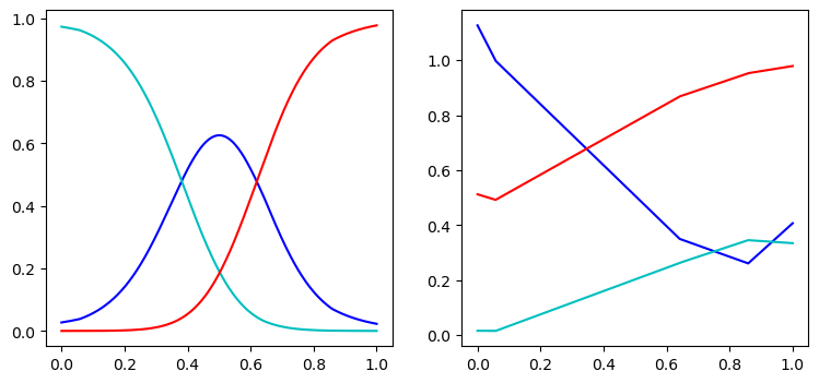
We also plot the approximate conditional modes, given by the mean of the most probable component $\mu(\textbf{x})=\mu_{\text{argmax}{\pi_k}(\textbf{x})}$ below:

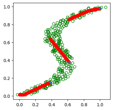
Note the resulting prediction is much more accurate compared to our original unimodal prediction, as desired.

General Case

In this blog post, we focused mainly on Gaussian Mixture Density networks with isotropic Gaussians. This can be extended to general covariance matrices $\Sigma_k(\textbf{x}$ using the Cholesky Factorization (see [2] and [5]). This gives a predictive distribution of $$p(\textbf{t}|\textbf{x}) = \sum_{k=1}^{K} \pi_k(\textbf{x})\mathcal{N}(\textbf{t}|\mu_k(\textbf{x}), \Sigma_k(\textbf{x}))$$ The training objective then becomes to minimize the negative log likelihood $$E(\textbf{w})=-\sum_{n=1}^{N}\ln{p_{\theta}(\textbf{t}_n|\textbf{x}_n)} \propto -\sum_{n=1}^{N}\ln\left\{\sum_{k=1}^{K} \pi_k(\textbf{x}_n)\exp\left(-\frac{1}{2}(\textbf{t}_n-\mu_k)^{T}\Sigma_k(\textbf{t}_n-\mu_k)-\frac{1}{2}\ln|\Sigma_k|\right)\right\}$$ $$= -\sum_{n=1}^{N}\text{LSE}_k\left(\ln\pi_k(\textbf{x}_n) -\frac{1}{2}(\textbf{t}_n-\mu_k)^{T}\Sigma_k(\textbf{t}_n-\mu_k)-\frac{1}{2}\ln|\Sigma_k| \right)$$ where $\text{LSE}$ is the LogSumExp. An excellent general tensorflow implementation of the general case writen by Axel Brando can be found here.

Full code for plotting and other details for the density network shown in this blog post can be found in my github in the corresponding repository.

References

[1] Brando, A, Mixture Density Networks implementation for distribution and uncertainty estimation, (2016), Github Repository
[2] Bishop, C. M. Mixture density networks. (1994).
[3] Bishop, C. M. Deep Learning: Foundations and Concepts (2024) Springer
[4] A. DasGupta, Asymptotic Theory Of Statistics And Probability. New York: Springer, 200
[5] Williams, P. M. (1996). Using neural networks to model conditional multivariate densities. Neural Comput., 8(4), 843–854